Vignette 1 - Inter-island distances
1. Isolation-by-distance in the Caribbean Flightless Ground Crickets
Papadopoulou & Knowles (2015) studied the effects of Pleistocene-era island connectivity on the genetic differentiation patterns of Carribbean flightless cricket (Amphiacusta sanctaecrucis) populations in the Virgin Islands, and found that population divergence times broadly correlate with a period of fluctuating sea levels and inter-island land bridge connections (~75-115 kya). In addition, the study found that all Virgin Island populations appear to exhibit a pattern of isolation-by-distance, with the exception of populations from St. Croix, athough these analyes were based on present-day Euclidean distances between populations. Using PleistoDist, it is possible to replicate the landscape genetic analyses, but with geographical distance matrices that account for sea level change over time.
For the purposes of this vignette, we will be reading and writing all files from a temporary directory, which we will assign to the variable called ’temp’ with the following code:
#generate temporary directory
temp <- file.path(tempdir())
To generate maps of sea level change over time, we first need to obtain a bathymetry map of the area of interest. In this vignette, we will use data from the GEBCO database (https://www.gebco.net/). In order to accurately estimate the sizes and distances of islands during periods of low sea level, it is important that the bathymetry map encompass as much of the local shelf as possible.
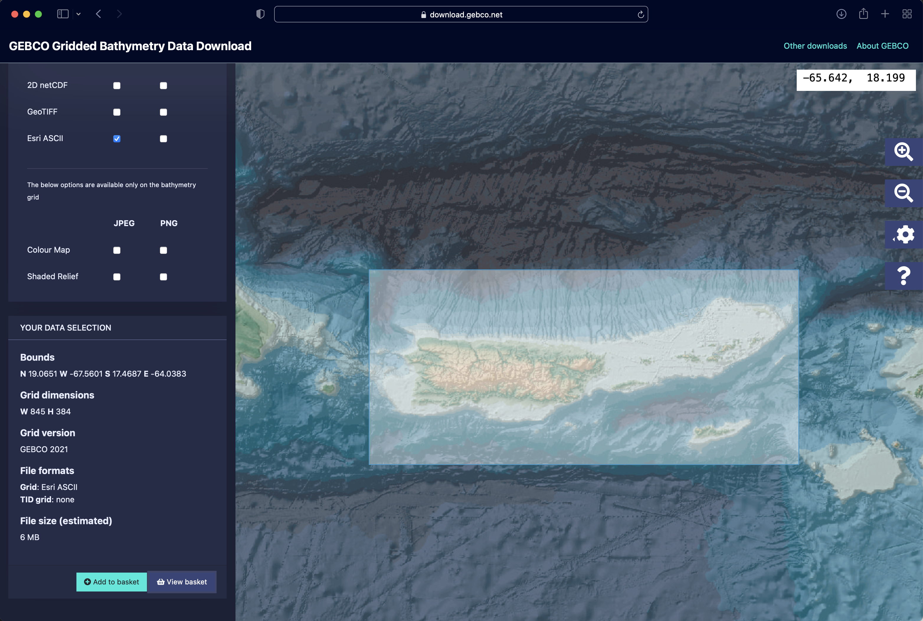
Once we have the bathymetry data downloaded and saved to the temporary directory as the file “VirginIslands.asc”, we can proceed to with generating the interval file as well as maps of island extents over time. To account for the most recently diverged island population on St. Croix, we set a time cutoff at 20 kya, at a maximum temporal resolution of 20 time intervals.
library(spaa)
library(dplyr)
library(PleistoDist)
library(vegan)

#generate interval file, with a time cutoff of 20 kya and 20 time intervals, using default sea level reconstruction from Bintanja & Van der Waal (2008)
getintervals_time(time = 20,intervals = 20,outdir = temp, sealvl = PleistoDist:::bintanja_vandewal_2008)

#generate map files
makemaps(inputraster = paste0(temp,"/VirginIslands.asc"), epsg = 32161, intervalfile = paste0(temp,"/intervals.csv"), offset = 0)
To visualise how the island system has changed over time as a result of sea level change, we can use the magick package in R to create an animated GIF file.
library(magick)
library(purrr)
library(gtools)
mixedsort(list.files(path=paste0(temp,"/raster_flat/"),pattern="*.tif",full.names=T)) %>%
  map(image_read) %>%
  image_join() %>%
  image_animate(fps=2) %>%
  image_write(paste0(temp,"/virginislands_animated.gif"))

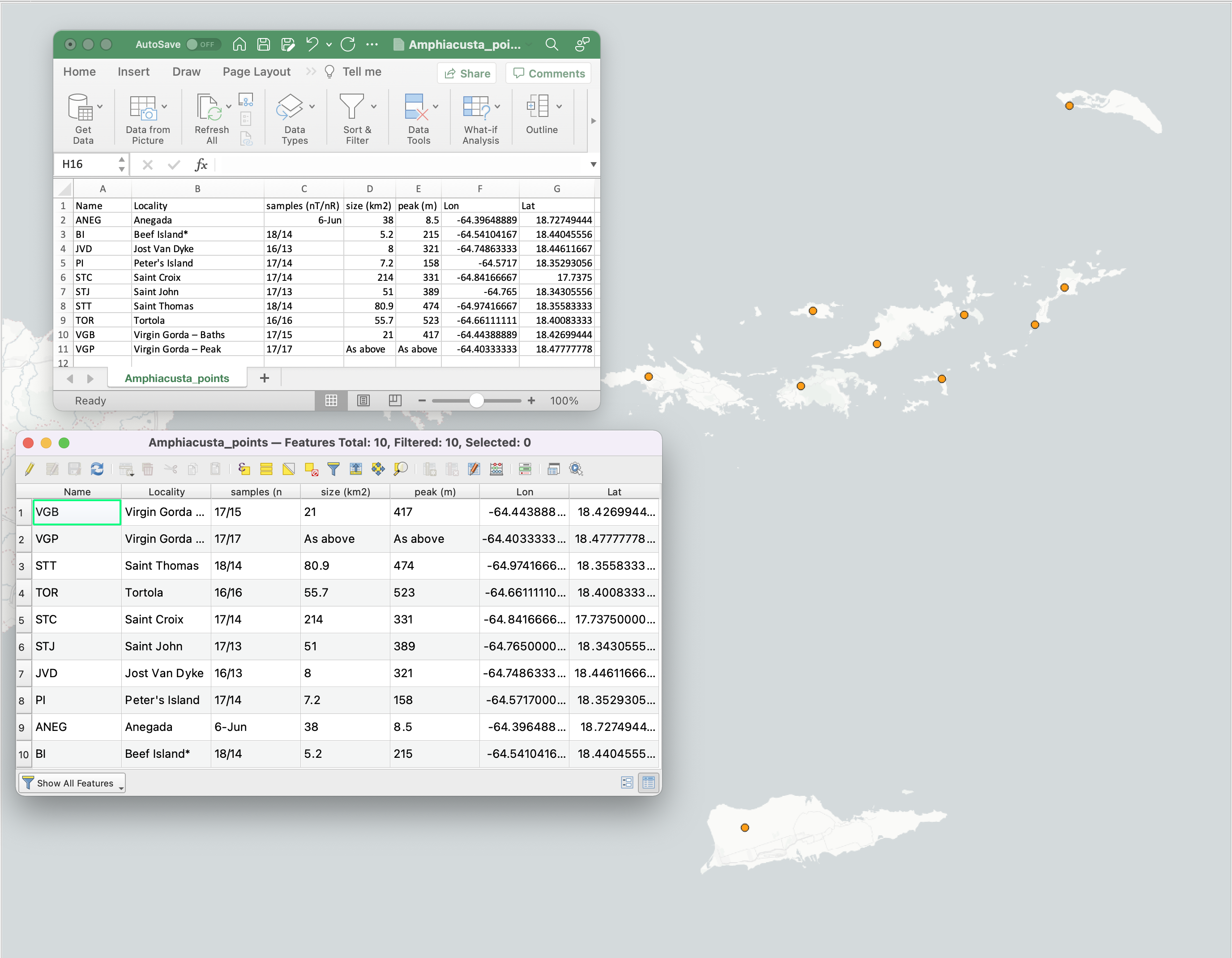
Now that the interval file and island maps have been generated, we need to generate a shapefile of points corresponding to our sampling localities. You can do this by importing a CSV file of coordinates into QGIS using the “Add Delimited Text Layer” function and exporting the file to the ’temp’ directory using the “Save Features As…” function. Remember to add a “Name” column with unique identifiers to the data table for each sampling point.
We can now use PleistDist to calculate various inter-island distance estimates. This step may take a while depending on the number of sampling points and time intervals defined.
#generate geographical distance matrices
pleistodist_euclidean(points = paste0(temp,"/Amphiacusta_points.shp"), epsg = 32161, outdir = temp)
pleistodist_leastcost(points = paste0(temp,"/Amphiacusta_points.shp"), epsg = 32161, intervalfile = paste0(temp,"/intervals.csv"), mapdir = temp, outdir = temp)
pleistodist_leastshore(points = paste0(temp,"/Amphiacusta_points.shp"), epsg = 32161, intervalfile = paste0(temp,"/intervals.csv"), mapdir = temp, outdir = temp)
pleistodist_centroid(points = paste0(temp,"/Amphiacusta_points.shp"), epsg = 32161, intervalfile = paste0(temp,"/intervals.csv"), mapdir = temp, outdir = temp)
pleistodist_meanshore(points = paste0(temp,"/Amphiacusta_points.shp"), epsg = 32161, intervalfile = paste0(temp,"/intervals.csv"), mapdir = temp, outdir = temp, maxsamp = 1000)
After calculating the geographical distance matrices, we can run Mantel tests and distance-based redundancy analyses (dbRDA) to assess the correlation between genetic distance and different forms of geographic distance estimation. $F_{ST}$ values for these analyses can be obtained from the bottom diagonal of Table S3 in the Supplementary Material of Papadopoulou and Knowles (2015).
#load FST distance matrix
gendist <- read.csv(paste0(temp,"/FST.csv")) %>%
  dplyr::select(Island1,Island2,FST) %>%
  spaa::list2dist()

#load and reshape geographic distance matrices to wide format
euclideandist <- read.csv(paste0(temp,"/island_euclideandist.csv")) %>%
  dplyr::select(Island1,Island2,interval0) %>%
  spaa::list2dist()

leastcostdist <- read.csv(paste0(temp,"/island_leastcostdist.csv")) %>%
  dplyr::select(Island1,Island2,mean) %>%
  spaa::list2dist()

leastshoredist <- read.csv(paste0(temp,"/island_leastshoredist.csv")) %>%
  dplyr::select(Island1,Island2,mean) %>%
  spaa::list2dist()

centroiddist <- read.csv(paste0(temp,"/island_centroiddist.csv")) %>%
  dplyr::select(Island1,Island2,mean) %>%
  spaa::list2dist()

meanshoredist1 <- read.csv(paste0(temp,"/island_meanshoredist.csv")) %>%
  dplyr::select(Island1,Island2,mean) %>%
  reshape(direction = "wide",idvar = "Island2",timevar = "Island1")

#since the mean shore-to-shore distance matrix is asymmetric, we need to calculate the average of the upper and lower triangles
meanshoredist1 <- meanshoredist1[,-1]
meanshoredist2 <- matrix(NA,ncol=ncol(meanshoredist1),nrow=nrow(meanshoredist1))
meanshoredist2[lower.tri(meanshoredist2)] <- rowMeans(cbind(meanshoredist1[upper.tri(meanshoredist1,diag=FALSE)],meanshoredist1[lower.tri(meanshoredist1,diag=FALSE)]))
meanshoredist2 <- as.dist(meanshoredist2)

#perform Mantel tests
euclideanmantel <- mantel(euclideandist,gendist/(1-gendist),permutations = 1000000)
leastcostmantel <- mantel(leastcostdist,gendist/(1-gendist),permutations = 1000000)
leastshoremantel <- mantel(leastshoredist,gendist/(1-gendist),permutations = 1000000)
centroidmantel <- mantel(centroiddist,gendist/(1-gendist),permutations = 1000000)
meanshoremantel <- mantel(meanshoredist2,gendist/(1-gendist),permutations = 1000000)

#perform dbRDA analyses
euclideanrda <- anova.cca(capscale(gendist/(1-gendist) ~ pcnm(euclideandist)$vectors),permutations=1000000)
leastcostrda <- anova.cca(capscale(gendist/(1-gendist) ~ pcnm(leastcostdist)$vectors),permutations=1000000)
leastshorerda <- anova.cca(capscale(gendist/(1-gendist) ~ pcnm(leastshoredist)$vectors),permutations=1000000)
centroidrda <- anova.cca(capscale(gendist/(1-gendist) ~ pcnm(centroiddist)$vectors),permutations=1000000)
meanshorerda <- anova.cca(capscale(gendist/(1-gendist) ~ pcnm(meanshoredist2)$vectors),permutations=1000000)
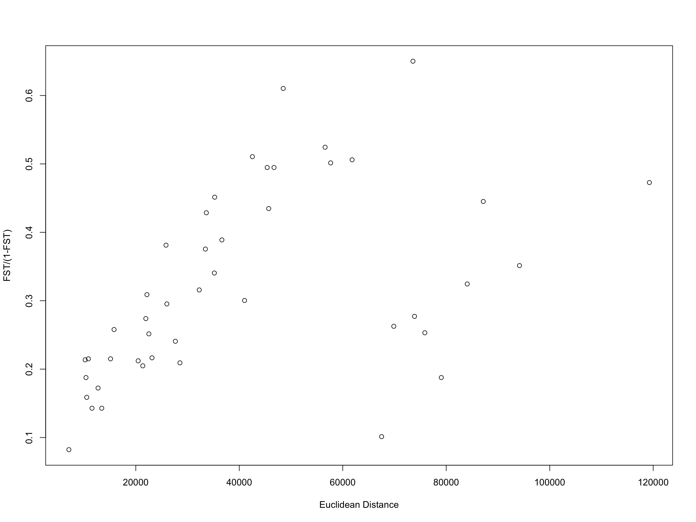
Similar to Papadopoulou & Knowles (2015), the results of the Mantel tests show that there is no significant correlation between genetic distance and Euclidean distance ($R^2$ = 0.228273, p = 0.0521429) when all populations are included in the analysis (See table below). In our extended analysis, none of the other geographic distance metrics show any significant correlation with genetic distance for Amphiacusta sanctaecrucis populations in the Virgin Islands. However, it is important to remember that Mantel tests are highly susceptible to spatial autocorrelation, and given the broad range of inter-population distances across this system (~7-120 km), it is possible that spatial autocorrelation may lead to non-linear genetic variation across geographic space.
plot(x = euclideandist, y = gendist/(1-gendist),xlab="Euclidean Distance",ylab="FST/(1-FST)")
As such, distance-based redundancy analyses may be more reliable for assessing the correlation between genetic and geographic distance. Interestingly, the dbRDA results indicate that both the least shore-to-shore and centroid-to-centroid distance matrices show highly significant correlations with genetic distance (p = 0.00661 and 0.007043, respectively), while Euclidean distance shows a somewhat significant correlation with genetic distance (p = 0.034779). Further model selection suggests that the centroid-to-centroid distance results in the best model fit to the data. This suggests that the genetic divergence patterns in Amphiacusta sanctaecrucis populations over the last 20,000 years are likely structured by broad-scale isolation-by-distance driven by inter-island overwater dispersal, rather than by land bridge-constrained dispersal. Although the results of this reanalysis need further validation, they nonetheless highlight the utility of time-normalised distance matrices for testing different hypotheses of dispersal across tropical island archipelagoes.
| Distance Type | Mantel $R^2$ | Mantel p-value | dbRDA $R^2_{adj}$ | dbRDA p-value |
|---|---|---|---|---|
| Euclidean Distance | 0.228273 | 0.0521429 | 0.3509484 | 0.034779 |
| Least Cost Distance | 0.2203824 | 0.0521409 | 0.1387593 | 0.3025617 |
| Least Shore-to-shore Distance | 0.0426482 | 0.1997118 | 0.4736347 | 0.00661 |
| Centroid-to-centroid Distance | 0.0090014 | 0.2004748 | 0.5933486 | 0.007043 |
| Mean Shore-to-shore Distance | 0.0035279 | 0.2976187 | -0.4337182 | 0.9366181 |
#model selection

#define upper and lower scope for model selection
upr <- capscale(gendist/(1-gendist) ~ pcnm(euclideandist)$vectors+pcnm(leastcostdist)$vectors+pcnm(leastshoredist)$vectors+pcnm(centroiddist)$vectors+pcnm(meanshoredist2)$vectors)
lwr <- capscale(formula = gendist/(1-gendist) ~ 1)

#run stepwise model selection and infer best-fit model
summary(ordistep(lwr,upr,trace=FALSE))
References
- Papadopoulou A, Knowles LL. 2015. Genomic tests of the species-pump hypothesis: Recent island connectivity cycles drive population divergence but not speciation in Caribbean crickets across the Virgin Islands. Evolution [Internet] 69:1501–1517. Available from: http://dx.doi.org/10.1111/evo.12667