Using PleistoDist

This short vignette will introduce you to the basic PleistoDist workflow, from generating the interval file, to plotting island maps, to calculating island metrics normalised over Pleistocene time. You should be able to run all of this code within R after installing the PleistoDist package without having to download any further data files.

Setting up the work environment

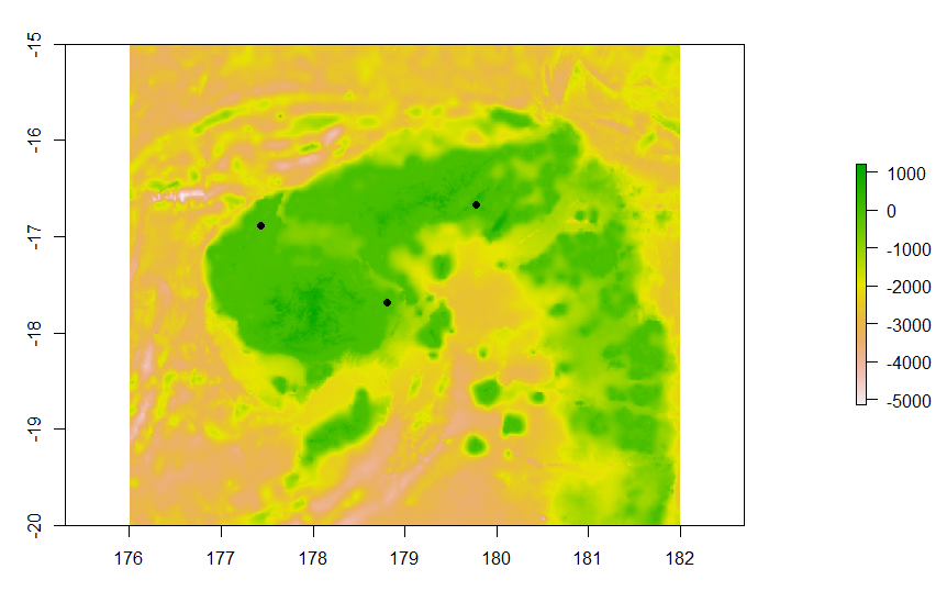
Before we begin our analysis, we first have to set up our working environment and load in the necessary files for this analysis. For the purposes of this tutorial, we will be exploring the impact of Pleistocene sea-level change on three islands in the Fijian archipelago: Nacula, Ovalau, and Vanua Levu. We will be using a bathymetry file of the Fijian archipelago from Darwell et al (2020), originally downloaded from the GEBCO database (https://www.gebco.net/), which has been included in the PleistoDist package.

library(sf)
library(terra)
library(raster)
library(PleistoDist)

#set temporary working directory 
path <- file.path(tempdir())

#load path to bathymetry file (this is included in the PleistoDist package)
fiji <- system.file("extdata","FJ.asc",package="PleistoDist")

#create shapefile of 3 points, one on each island of interest
testpoints <- st_multipoint(rbind(c(177.43035,-16.88739), #Nacula
                                  c(178.81200,-17.68200), #Ovalau
                                  c(179.77684,-16.66527))) #Vanua Levu

#visualise bathymetry map and points
plot(raster(fiji))
points(testpoints,pch=19)

Figure 1: Bathymetry map of Fiji, with points corresponding to the three islands of interest (Nacula, Ovalau, Vanua Levu).

#convert island points to feature geometry
testpoints <- st_sfc(testpoints) %>%
  st_cast("POINT")

#set default projection of WGS84 for island points
st_crs(testpoints) = 4326

#reproject points to EPSG:3141 (Fiji) and write to file
testpoints_proj <- st_transform(testpoints,3141)
write_sf(testpoints_proj,paste0(path,"/testpoints.shp"))

Note that because the shapefile of points used in this example does not have a ‘Name’ column, all PleistoDist outputs will use the FID value of each point by default. You can, however, modify the shapefile’s attribute table to include a ‘Name’ column, which PleistoDist will use instead of FID values.

Generate interval file and maps

Now that the working environment has been set up, we can proceed with using PleistoDist to generate the interval file as well as the maps of island extents. For this analysis, we will be setting a cutoff time of 20 kya (the approximate time of the the last glacial maximum), for 10 time bin intervals, using the default sea-level reconstruction by Bintanja and Van de Wal (2008). We will also assume no net uplift or subsidence of the archipelago when generating the island maps (i.e. the offset parameter in the makemaps() function will be set to 0). All output files are automatically saved to the specified output folder (parameter: outdir).

#generate interval file, with a cutoff time of 20kya and binning by sea-level, for 10 sea-level bins
getintervals_sealvl(time = 20,
                    intervals = 10,
                    outdir = path,
                    sealvl = PleistoDist:::bintanja_vandewal_2008) #optional, default bintanja_vandewal_2008

#create maps
makemaps(inputraster = fiji,
         epsg = 3141,
         intervalfile = paste0(path,"/intervals.csv"),
         outdir=path,
         offset = 0) #optional, default = 0

Calculate island shape metrics

To estimate the perimeter, 2D area, and surface area of Nacula, Ovalau, and Vanua Levu islands over the last 20 kya, we can individually run each of the pleistoshape family of functions (pleistoshape_perimeter(), pleistoshape_area(), pleistoshape_surfacearea()), or we can just use the pleistoshape_all() function to run all three calculations at the same time. The results of these functions are saved in the output directory specified by the ‘outdir’ parameter.

#calculate all island shape metrics (area, surface area, perimeter)
pleistoshape_all(points= paste0(path,"/testpoints.shp"),
                 epsg = 3141,
                 intervalfile = paste0(path,"/intervals.csv"),
                 mapdir = path,
                 outdir = path)

#View island area output
islandarea <- read.csv(paste0(path,"/island_area.csv"))
View(islandarea)

Table 1: 2D area of each Fijian island (0: Nacula, 1: Ovalau, 2: Vanua Levu) for each time interval, as well as the mean island area normalised over Pleistocene time.

Island	interval0	interval1	interval2	interval3	interval4	interval5	interval6	interval7	interval8	interval9	interval10	mean
0	93302544.65	898949734.5	1857126302	17411066158	19148927468	20392690954	21244583753	21661605561	22066457472	22252251235	22433988366	11287852047
1	129812236	194718354	13841229667	17411066158	19148927468	20392690954	21244583753	21661605561	22066457472	22252251235	22433988366	12270324007
2	6097929788	6655311076	8314473718	11150871075	13700870187	15089049786	16262227869	16817986504	17278008616	17978994690	18310827219	11770663955

Calculate inter-island and inter-point distances

To calculate inter-island distances, you can choose between three different types of inter-island distance metric. To calclulate centroid-to-centroid distances, use the pleistodist_centroid() function. Least shore-to-shore distances can be calculated using the pleistodist_leastshore() function, while mean shore-to-shore distances can be calculated using the pleistodist_meanshore() function. To calculate distances between points, you can opt to calculate the Euclidean distance (i.e. straight line distance) or the least cost path between each pair of points. Note that since Euclidean distances are static and not affected by sea level change, it will only be reported for one time/sea level interval. All outputs from these functions will be saved to the directory specified by the ‘outdir’ parameter.

#calculate Euclidean distance between points
pleistodist_euclidean(points = paste0(path,"/testpoints.shp"),
                      epsg = 3141,
                      outdir = path)

#calculate inter-island centroid-to-centroid distance
pleistodist_centroid(points = paste0(path,"/testpoints.shp"),
                     epsg = 3141,
                     intervalfile = paste0(path,"/intervals.csv"),
                     mapdir = path,
                     outdir = path)

#calculate inter-island least shore-to-shore distance
pleistodist_leastshore(points = paste0(path,"/testpoints.shp"),
                       epsg = 3141,
                       intervalfile = paste0(path,"/intervals.csv"),
                       mapdir = path,
                       outdir = path)

#calculate inter-island mean shore-to-shore distance
pleistodist_meanshore(points = paste0(path,"/testpoints.shp"),
                       epsg = 3141,
                       intervalfile = paste0(path,"/intervals.csv"),
                       mapdir = path,
                       outdir = path,
                       maxsamp = 10000) #optional, the number of points to sample along the shoreline, default 1000

#calculate point-to-point least cost distance
pleistodist_leastcost(points = paste0(path,"/testpoints.shp"),
                       epsg = 3141,
                       intervalfile = paste0(path,"/intervals.csv"),
                       mapdir = path,
                       outdir = path)

Calculate inter-island net migration and inter-island visibility

PleistoDist also contains two higher-level functions that (1) estimate the ratio of migrants exchanged between a pair of islands (pleistodist_netmig(); based on a model by MacArthur and Wilson (1967)) as well as (2) the estimated visibility of a destination island relative to an observer located on a source island (pleistodist_visibility()). As with all other functions in PleistoDist, all outputs from these functions will be saved in CSV format in the directory specified by the ‘outdir’ parameter.

#calculate net inter-island migration
pleistodist_netmig(points = paste0(path,"/testpoints.shp"),
                   epsg = 3141,
                   disttype = "centroid", #can also be "leastshore" or "meanshore"
                   intervalfile = paste0(path,"/intervals.csv"),
                   mapdir = path,
                   outdir = path)

#calculate inter-island visbility
pleistodist_visibility(points = paste0(path,"/testpoints.shp"),
                      epsg = 3141,
                      intervalfile = paste0(path,"/intervals.csv"),
                      mapdir = path,
                      outdir = path,
                      height = 10, #default 0
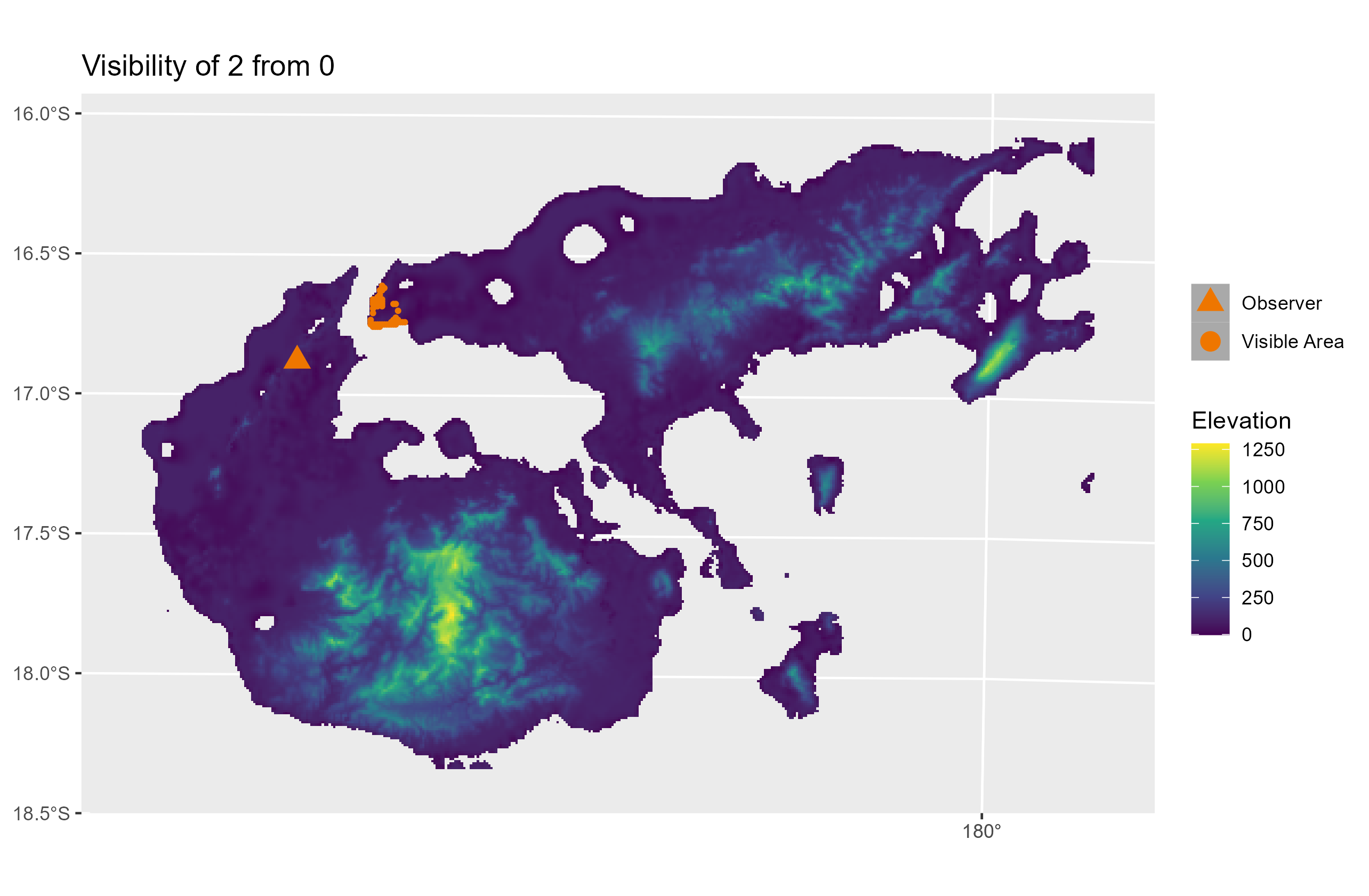
                      plotfigs = TRUE) #false by default. User will be prompted to confirm if number of points exceeds 5

The pleistodist_visibility() function can also plot maps of inter-island visibility if the ‘plotfigs’ parameter is set to TRUE. Users are warned, however, not to activate this parameter if the number of points is high, since PleistoDist may end up generating a large number of graphics files (e.g. an analysis with 5 points and 10 intervals will generate up to a theoretical maximum of 250 image files). Below is an example of what a visibility map looks like:

References

• Bintanja, R., & van de Wal, R. S. W. (2008). North American ice-sheet dynamics and the onset of 100,000-year glacial cycles. Nature, 454(7206), 869–872. https://doi.org/10.1038/nature07158
• Darwell, C. T., Fischer, G., Sarnat, E. M., Friedman, N. R., Liu, C., Baiao, G., Mikheyev, A. S., & Economo, E. P. (2020). Genomic and phenomic analysis of island ant community assembly. Molecular Ecology, 29(9), 1611–1627. https://doi.org/10.1111/mec.15326
• MacArthur R. H., & Wilson E. O. (1967). The Theory of Island Biogeography. Princeton, N.J.: Princeton University Press, 203 p.