Vignette 2 - Species-area relationships
2. Angiosperm species-area relationships in the Aegean Islands
Hammoud et al (2021) examined the relationship between island area and species richness in the Aegean Islands across multiple plant and animal taxa, taking into account historical sea level change over the Quaternary. They find that land-bridge islands, which were historically connected to the mainland, exhibit weaker correlations between island area and endemic species richness relative to true islands, which were never connected with the mainland. The results of this study suggest that periodic land bridge formation between islands and the mainland may inhibit the differentiation of insular populations. For the sake of this vignette, however, we will only be looking at species-area relationships for angiosperms on true islands in the Aegean archipelago.
For the purposes of this vignette, we will be reading and writing all files from a temporary directory, which we will assign to the variable called ’temp’ with the following code:
#generate temporary directory
temp <- file.path(tempdir())
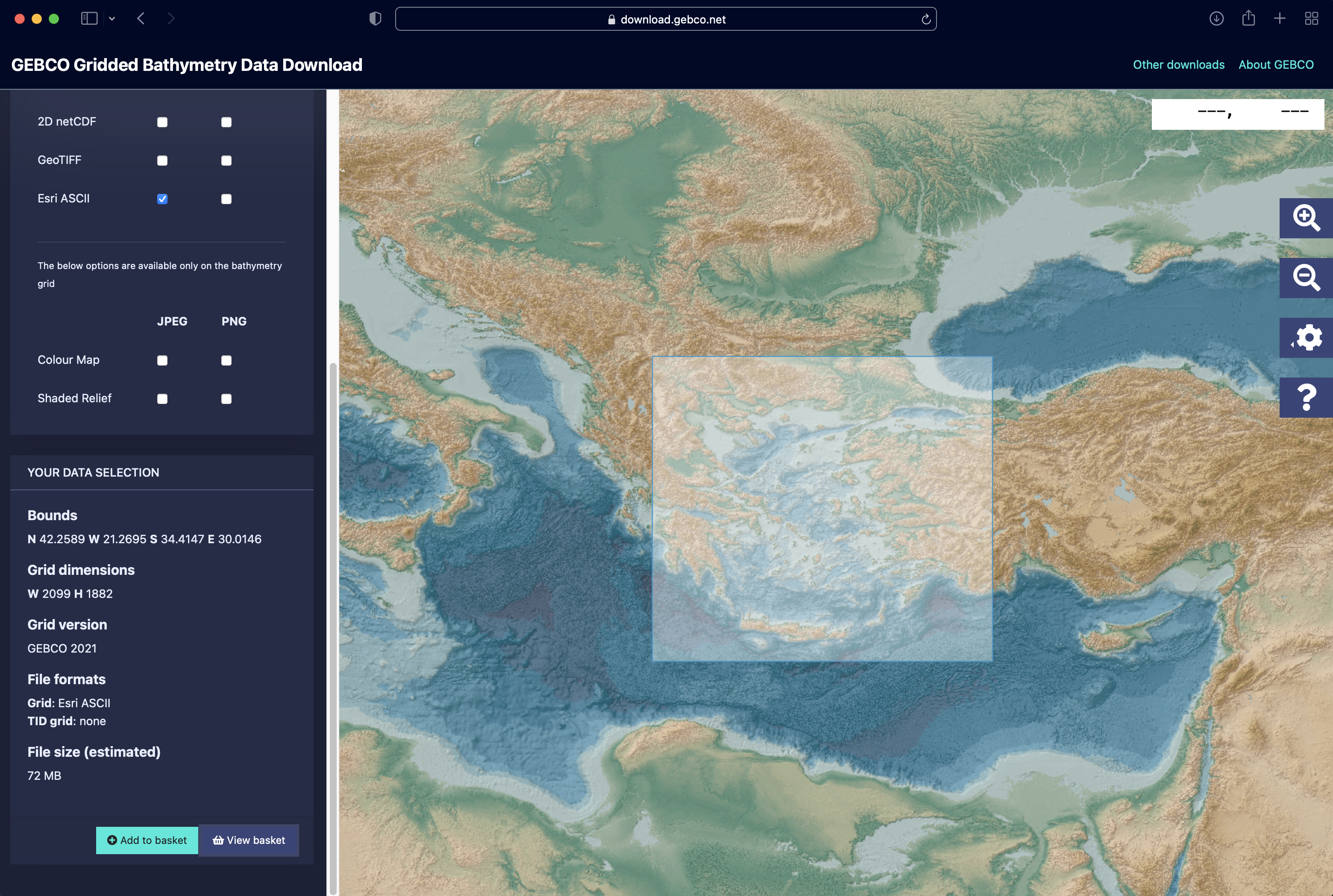
First, we need to download bathymetry data for the Aegean Islands. For this vignette, we will use data from the Generalised Bathymetric Chart of the Oceans (GEBCO: https://www.gebco.net/)
Now we can generate the interval file. For the sake of this demonstration, we will generate an interval file with sea level depth intervals (as opposed to time intervals). with a time cutoff of 20 kya (the approximate last glacial maximum) and 40 depth intervals (~3m per interval). We then use the makemaps() function to generate maps of island extents, using the projection EPSG:2100 (GGRS87/Greek Grid), assuming no overall uplift or subsidence of the study area (see Simaiakis et al (2017), however, for further discussion).
#generate interval file with a time cutoff of 20 kya (LGM), and 40 intervals (~3m per interval)
getintervals_sealvl(time = 20, intervals = 40, outdir = temp, sealvl = PleistoDist:::bintanja_vandewal_2008)

#generate maps of island extents
makemaps(inputraster = paste0(temp,"/AegeanIslands.asc"), epsg=2100, intervalfile = paste0(temp,"/intervals.csv"), outdir = temp, offset = 0)
We can visualise the effect of sea level change over the past 20,000 years by animating the maps generated by PleistoDist. Note that because we used sea level depth intervals to generate the interval file, this animation is not in chronological order.
library(magick)
library(purrr)
library(gtools)
mixedsort(list.files(path=paste0(temp,"/raster_flat/"),pattern="*.tif",full.names=T)) %>%
  map(image_read) %>%
  image_join() %>%
  image_animate(fps=2) %>%
  image_write(paste0(temp,"/aegeanislands_animated.gif"))
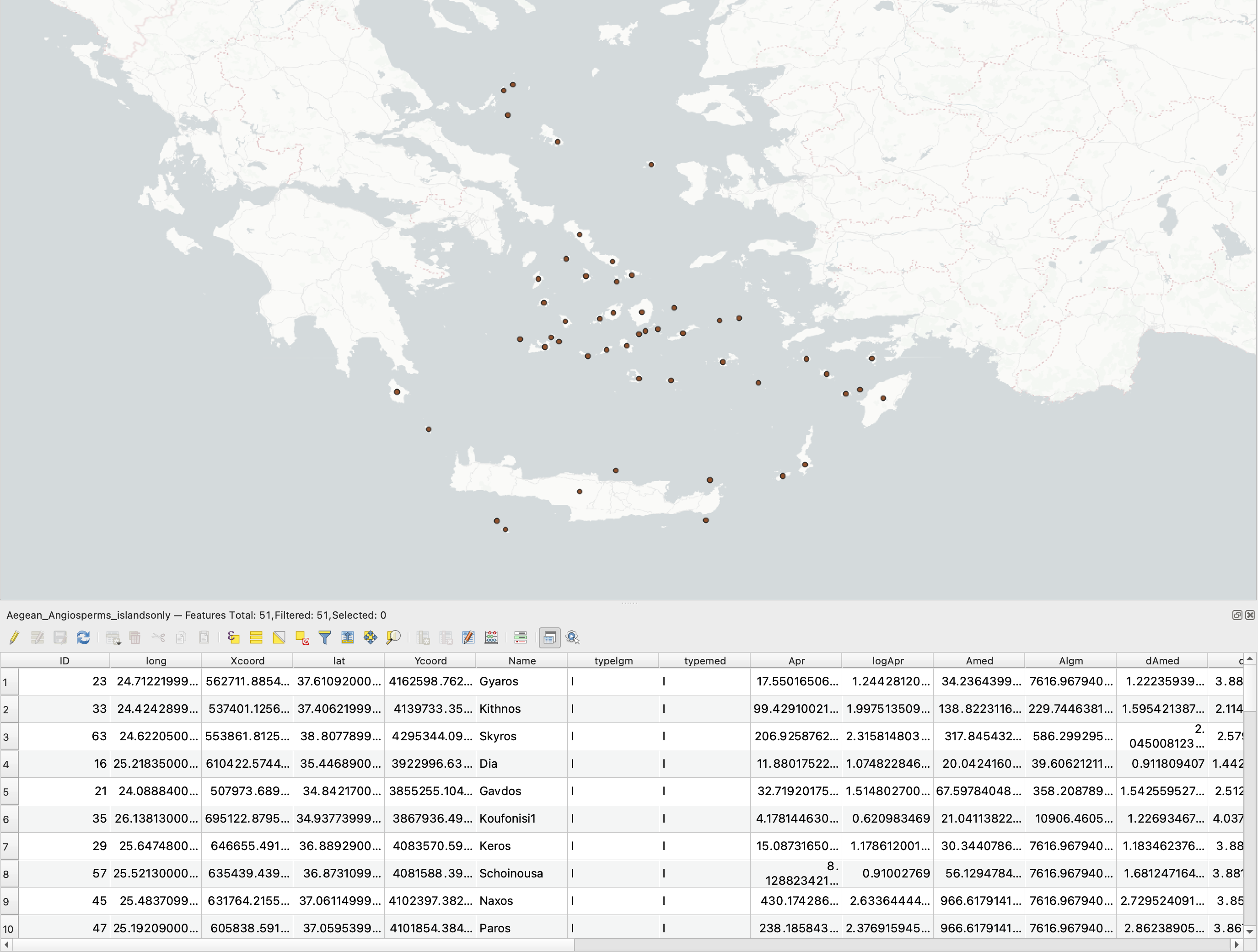
We need to generate a shapefile of sampling points for calculating island area over time. To do this, we will use the ‘Add Delimited Text Layer’ function in QGIS to read the Aegean_Angiosperms.csv file from the Hammoud et al (2021) Dryad dataset (https://datadryad.org/stash/dataset/doi:10.5061/dryad.dfn2z350z), rename the ‘Islands’ column to ‘Name’, and filter for rows where typelgm == I (filtering out islands that were previously connected to the mainland).
We can now use the pleistoshape functions in PleistoDist to calculate the island area for each sea level interval as well as the mean island area over time. To see if elevation plays a role in affecting species richness, we can also use PleistoDist to calculate the surface area of each island.
#calculate island area over time
pleistoshape_area(points = paste0(temp,"/Aegean_Angiosperms_islandsonly.shp"), epsg = 2100, intervalfile = paste0(temp,"/intervals.csv"), mapdir = temp, outdir = temp)
pleistoshape_surfacearea(points = paste0(temp,"/Aegean_Angiosperms_islandsonly.shp"), epsg = 2100, intervalfile = "output/intervals.csv", mapdir = temp, outdir = temp)
After calculating the mean island area and surface area, we can use simple linear models to assess the relationship between island area and species richness. We will exclude the island of Skantzoura since the sampling point fell outside the inferred island boundary for at least the first 6 intervals.
#load and filter PleistoDist outputs
islandarea <- read.csv(paste0(temp,"/island_area.csv")) %>%
  dplyr::select(Island,interval0,mean) %>%
  dplyr::filter(Island != "Skantzoura")
islandsurfacearea <- read.csv(paste0(temp,"/island_surfacearea.csv") %>%
  dplyr::select(Island,interval0,mean) %>%
  dplyr::filter(Island != "Skantzoura")

#load species richness dataset from Hammoud et al (2021) and rename island name column for consistency
angiosperms <- read.csv(paste0(temp,"/Aegean_angiosperms.csv"),sep = ";") %>%
  dplyr::select(island,Sn,Nn,En)
colnames(angiosperms)[1] <- "Island"

#join PleistoDist outputs with species richness data from Hammoud et al (2021) dataset
islandarea <- left_join(islandarea,angiosperms,by="Island")
islandsurfacearea <- left_join(islandsurfacearea,angiosperms,by="Island")

#run linear models
area_allsp <- lm(log(Sn) ~ log(mean),data=islandarea)
surfacearea_allsp <- lm(log(Sn) ~ log(mean),data=islandsurfacearea)
area_native <- lm(log(Nn) ~ log(mean),data=islandarea)
surfacearea_native <- lm(log(Nn) ~ log(mean),data=islandsurfacearea)
area_endemic <- lm(log(En) ~ log(mean),data=islandarea)
surfacearea_endemic <- lm(log(En) ~ log(mean),data=islandsurfacearea)
area_allsp_present <- lm(log(Sn) ~ log(interval0),data=islandarea)
surfacearea_allsp_present <- lm(log(Sn) ~ log(interval0),data=islandsurfacearea)
area_native_present <- lm(log(Nn) ~ log(interval0),data=islandarea)
surfacearea_native_present <- lm(log(Nn) ~ log(interval0),data=islandsurfacearea)
area_endemic_present <- lm(log(En) ~ log(interval0),data=islandarea)
surfacearea_endemic_present <- lm(log(En) ~ log(interval0),data=islandsurfacearea)
| Chorotype | Present day 2D Area $R^2_{adj}$ | p-value | AIC | Time-corrected 2D Area $R^2_{adj}$ | p-value | AIC |
|---|---|---|---|---|---|---|
| Total Species Richness | 0.7621572 | 8.5133133^{-17} | 22.043369 | 0.3917022 | 7.0415557^{-7} | 68.9961019 |
| Native Non-endemic Species Richness | 0.7445056 | 4.797213^{-16} | 26.3768068 | 0.3873976 | 8.3800519^{-7} | 70.1025982 |
| Endemic Species Richness | 0.4888763 | 9.8006389^{-9} | 81.6361191 | 0.2662759 | 7.4543655^{-5} | 99.7121938 |
| Chorotype | Present day Surface Area $R^2_{adj}$ | p-value | AIC | Time-corrected Surface Area $R^2_{adj}$ | p-value | AIC |
|---|---|---|---|---|---|---|
| Total Species Richness | 0.7605729 | 9.9934794^{-17} | 22.3753279 | 0.392509 | 6.8147118^{-7} | 68.9297401 |
| Native Non-endemic Species Richness | 0.7430394 | 5.508435^{-16} | 26.662924 | 0.3882024 | 8.1124869^{-7} | 70.0368659 |
| Endemic Species Richness | 0.4870423 | 1.0698232^{-8} | 81.8152045 | 0.2665386 | 7.3875836^{-5} | 99.6942878 |
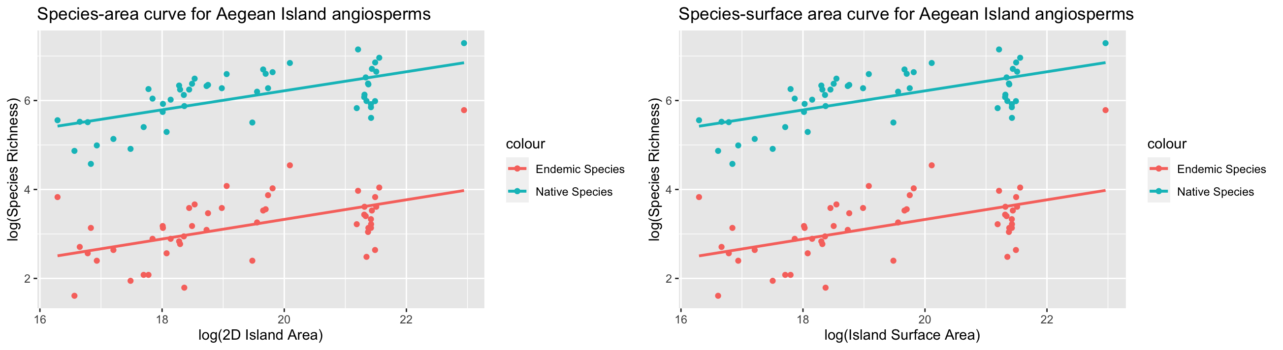
Simple linear models show that species-area relationships are significantly positively correlated for all angiosperm chorotypes across the true islands of the Aegean Sea, which is consistent with the findings of Hammoud et al (2021). However, contrary to the findings of Hammoud et al (2021) our extended analyses show that, based on the AIC values of each model, present-day 2D island area is the best predictor of angiosperm species richness for true islands, instead of time-corrected 2D area or surface area. While the models run in this reanalysis are relatively unsophisticated, they nonetheless suggest that species turnover on true islands may be relatively fast, resulting in a rapid equilibration of species richness to contemporary island areas. Alternatively, the eustatic sea-level reconstruction model used in this analaysis may have led to inaccurate reconstructions of Pleistocene island extents in the Aegean Sea, and more accurate isostatic models may be needed to better assess the relationship between species richness and island area in the Aegean Sea.
areaplot <- ggplot(islandarea)+
  geom_point(aes(x=log(mean),y=log(Nn),col="Native Species"))+
  geom_smooth(aes(x=log(mean),y=log(Nn),col="Native Species"),method="lm",se=FALSE)+
  geom_point(aes(x=log(mean),y=log(En),col="Endemic Species"))+
  geom_smooth(aes(x=log(mean),y=log(En),col="Endemic Species"),method="lm",se=FALSE)+
  labs(x="log(2D Island Area)", y = "log(Species Richness)", title = "Species-area curve for Aegean Island angiosperms")

surfaceareaplot <- ggplot(islandsurfacearea)+
  geom_point(aes(x=log(mean),y=log(Nn),col="Native Species"))+
  geom_smooth(aes(x=log(mean),y=log(Nn),col="Native Species"),method="lm",se=FALSE)+
  geom_point(aes(x=log(mean),y=log(En),col="Endemic Species"))+
  geom_smooth(aes(x=log(mean),y=log(En),col="Endemic Species"),method="lm",se=FALSE)+
  labs(x="log(Island Surface Area)", y = "log(Species Richness)", title = "Species-surface area curve for Aegean Island angiosperms")

ggarrange(areaplot,surfaceareaplot,ncol=2,nrow=1)
References
- Hammoud C. 2021. Past connections with the mainland structure patterns of insular species richness in a continental-shelf archipelago (Aegean Sea, Greece): Species richness matrixes and shapefiles. Dryad. Dataset. https://doi.org/10.5061/dryad.dfn2z350z
- Hammoud C, Kougioumoutzis K, Rijsdijk KF, Simaiakis SM, Norder SJ, Foufopoulos J, Georgopoulou E, Loon EE. 2021. Past connections with the mainland structure patterns of insular species richness in a continental‐shelf archipelago (Aegean Sea, Greece). Ecol. Evol. [Internet] 11:5441–5458. Available from: http://dx.doi.org/10.1002/ece3.7438
- Simaiakis SM, Rijsdijk KF, Koene EFM, Norder SJ, Van Boxel JH, Stocchi P, Hammoud C, Kougioumoutzis K, Georgopoulou E, Van Loon EE, Tjørve KMC, Tjørve E. 2017. Geographic changes in the Aegean Sea since the Last Glacial Maximum: Postulating biogeographic effects of sea-level rise on islands. Palaeogeogr. Palaeoclimatol. Palaeoecol. 471:108–119.