Vignette 3 - Net inter-island migration

3. Inter-island migration in Horornis Bush Warblers across the Fijian Archipelago

One of the predictions of the Theory of Island Biogeography (MacArthur & Wilson, 1967) is that the relative rate of migration between island pairs can be predicted by the size, relative orientation, and distance of the source islands. Gyllenhaal et al (2020) test this expectation by estimating the rates of inter-island migration in the Fiji Bush Warbler (Horornis ruficapilla) between four large islands across the Fijian archipelago, concluding that rates of inter-island migration are consistent with the neutral expectations of MacArthur & Wilson. This neutral expectation can now be easily calculated using PleistoDist, while taking into account the effect of sea level change over Pleistocene time.

For the purposes of this vignette, we will be reading and writing all files from a temporary directory, which we will assign to the variable called ’temp’ with the following code:

#generate temporary directory
temp <- file.path(tempdir())

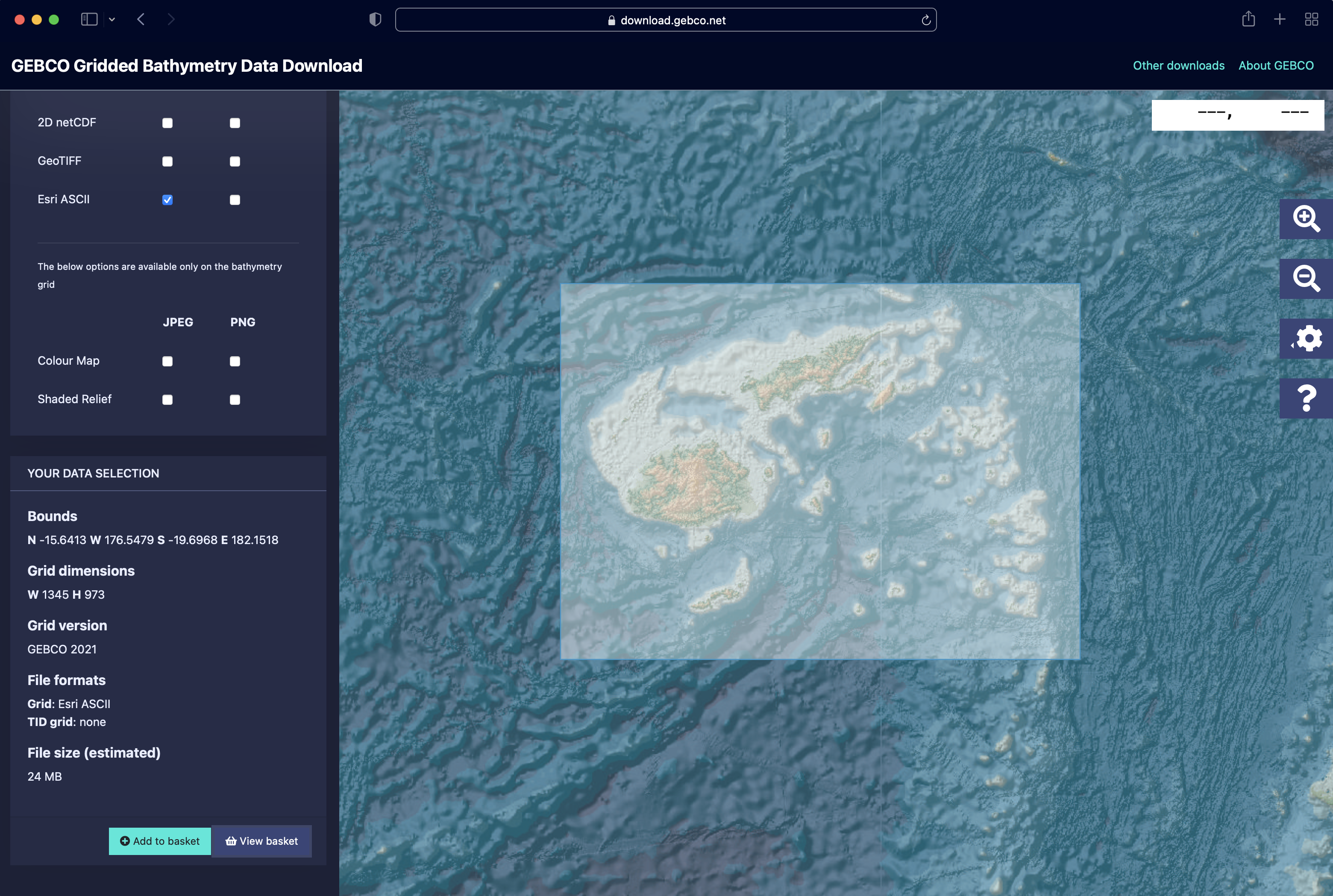
The first step in this analysis is to download bathymetry data for the area of interest. For this vignette, we will be downloading a bathymetric map of the Fijian archipelago from the Generalised Bathymetric Chart of the Oceans (GEBCO: https://www.gebco.net/).

We will also need to generate the interval file, which converts sea level change into a series of discrete intervals. In this analysis, we will use a time cutoff of 115 kya, corresponding with the start of the last glacial period, for 40 sea level depth intervals. Once the interval file has been generated, we can use the makemaps() function to generate maps of island extents over time.

#generate interval file for cutoff time of 115 kya (onset of last glacial period), for 40 sea level depth intervals
getintervals_sealvl(time = 115, intervals = 40, outdir = temp, sealvl = PleistoDist:::bintanja_vandewal_2008)

#generate maps of island extents
makemaps(inputraster = paste0(temp,"/Fiji.asc"), epsg = 3141, intervalfile = paste0(temp,"/intervals.csv"), outdir = temp, offset = 0)

We can use the R package magick to stitch the maps of island extent into an animation of sea level change over time. Note that because we generated intervals by sea level depth, this animation is not in chronological order.

library(magick)
library(purrr)
library(gtools)
mixedsort(list.files(path=paste0(temp,"/raster_flat/"),pattern="*.tif",full.names=T)) %>% 
  map(image_read) %>% 
  image_join() %>% 
  image_animate(fps=2) %>% 
  image_write(paste0(temp,"/fiji_animated.gif"))

We will also need to generate a shapefile of sampling points, which PleistoDist will use to identify pairs of islands for calculating relative net migration. I recommend using the ‘Create Layer > New Shapefile Layer’ function in QGIS, not forgetting to add a ‘Name’ column with unique island identifiers, and exporting the points layer in .SHP format.

Once all that has been set up, we can proceed to run the net migration function in PleistoDist. The software will automatically detect if the necessary distance matrix and area files are in the output folder, and will generate the missing files if needed.

#calculate net inter-island migration over time
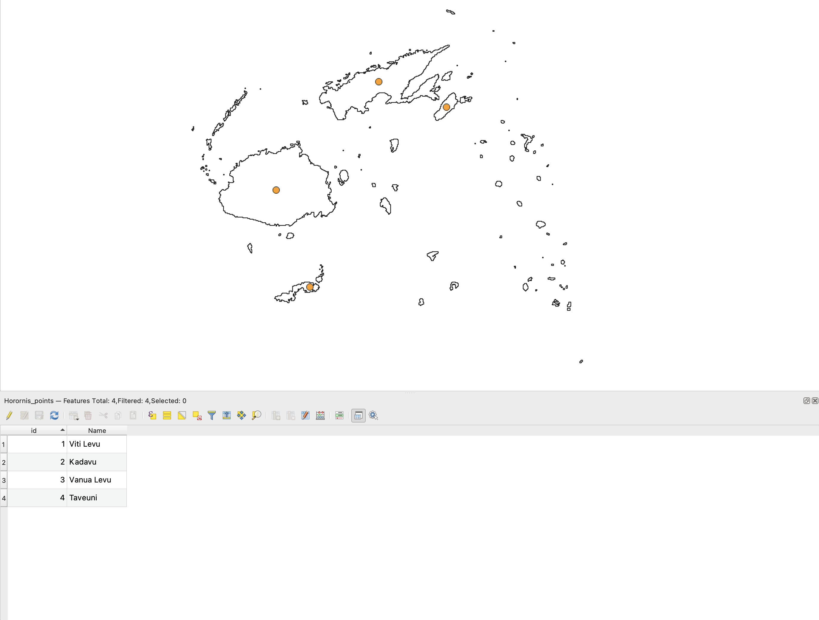
pleistodist_netmig(points = paste0(temp,"/Horornis_points.shp"), epsg = 3141, disttype = "centroid", intervalfile = paste0(temp,"/intervals.csv"), mapdir = temp, outdir = temp)
pleistodist_netmig(points = paste0(temp,"/Horornis_points.shp"), epsg = 3141, disttype = "leastshore", intervalfile = paste0(temp,"/intervals.csv"), mapdir = temp, outdir = temp)
pleistodist_netmig(points = paste0(temp,"/Horornis_points.shp"), epsg = 3141, disttype = "meanshore", intervalfile = paste0(temp,"/intervals.csv"), mapdir = temp, outdir = temp)

Now we can run some simple analyses to compare the empirical estimates of inter-island gene flow (obtained from the associated GitHub repository: https://github.com/ethangyllenhaal/horornis_UCE/blob/master/R_scripts/horornis_geneflow_comp.csv) with the PleistoDist-generated expectations.

#load interval file for calculating parameter standard deviation, extract time durations of each interval as weights
intervalfile <- read.csv(paste0(temp,"/intervals.csv"))
wts <- intervalfile$TimeInterval

#load net migration estimates, calculate the weighted standard deviation for the mean, and import empirical data
netmig_centroid <- read.csv(paste0(temp,"/island_netmigration_centroid.csv")) %>%
  drop_na() %>% 
  rowwise() %>%
  mutate(stdev = sqrt(wtd.var(c_across(interval0:interval40),wts))) %>%
  mutate(low = mean - qt(0.975,df=sum(wts)-1)*stdev/sqrt(sum(wts))) %>%
  mutate(upp = mean + qt(0.975,df=sum(wts)-1)*stdev/sqrt(sum(wts))) %>%
  dplyr::select(Island1,Island2,mean,stdev,low,upp) %>%
  mutate(Method = "Centroid (115 kya)")
netmig_leastshore <- read.csv(paste0(temp,"/island_netmigration_leastshore.csv")) %>%
  drop_na() %>% 
  rowwise() %>%
  mutate(stdev = sqrt(wtd.var(c_across(interval0:interval40),wts))) %>%
  mutate(low = mean - qt(0.975,df=sum(wts)-1)*stdev/sqrt(sum(wts))) %>%
  mutate(upp = mean + qt(0.975,df=sum(wts)-1)*stdev/sqrt(sum(wts))) %>%
  dplyr::select(Island1,Island2,mean,stdev,low,upp) %>%
  mutate(Method = "LeastShore (115 kya)")
netmig_meanshore <- read.csv(paste0(temp,"/island_netmigration_meanshore.csv")) %>%
  drop_na() %>% 
  rowwise() %>%
  mutate(stdev = sqrt(wtd.var(c_across(interval0:interval40),wts))) %>%
  mutate(low = mean - qt(0.975,df=sum(wts)-1)*stdev/sqrt(sum(wts))) %>%
  mutate(upp = mean + qt(0.975,df=sum(wts)-1)*stdev/sqrt(sum(wts))) %>%
  dplyr::select(Island1,Island2,mean,stdev,low,upp) %>%
  mutate(Method = "MeanShore (115 kya)")
netmig_centroid_presentday <- read.csv(paste0(temp,"/island_netmigration_centroid.csv")) %>%
  dplyr::select(Island1,Island2,interval0) %>%
  rename(mean = interval0) %>%
  drop_na() %>%
  mutate(stdev=0,low=mean,upp=mean,Method="Centroid (Present Day)")
netmig_leastshore_presentday <- read.csv(paste0(temp,"/island_netmigration_leastshore.csv")) %>%
  dplyr::select(Island1,Island2,interval0) %>%
  rename(mean = interval0) %>%
  drop_na() %>%
  mutate(stdev=0,low=mean,upp=mean,Method="LeastShore (Present Day)")
netmig_meanshore_presentday <- read.csv(paste0(temp,"/island_netmigration_meanshore.csv")) %>%
  dplyr::select(Island1,Island2,interval0) %>%
  rename(mean = interval0) %>%
  drop_na() %>%
  mutate(stdev=0,low=mean,upp=mean,Method="MeanShore (Present Day)")
netmig_all <- bind_rows(netmig_centroid,netmig_leastshore,netmig_meanshore,netmig_centroid_presentday,netmig_leastshore_presentday,netmig_meanshore_presentday) %>%
  filter((Island1 == "Taveuni" && Island2 == "Vanua Levu") || (Island1 == "Kadavu" && Island2 == "Viti Levu") || (Island1 == "Viti Levu" && Island2 == "Vanua Levu")) %>%
  add_row(Island1="Taveuni",Island2="Vanua Levu",mean=0.19388384,stdev=NA,low=0.173360085,upp=0.214407595,Method="Empirical") %>%
  add_row(Island1="Kadavu",Island2="Viti Levu",mean=0.007390666,stdev=NA,low=0.006692428,upp=0.008088905,Method="Empirical") %>%
  add_row(Island1="Viti Levu",Island2="Vanua Levu",mean=1.093240119,stdev=NA,low=0.456999638,upp=1.729480601,Method="Empirical") %>%
  add_row(Island1="Taveuni",Island2="Vanua Levu",mean=0.139053468,stdev=NA,low=0.122602818,upp=0.155504118,Method="Empirical NoAdmix") %>%
  add_row(Island1="Kadavu",Island2="Viti Levu",mean=0.262898923,stdev=NA,low=0.035465968,upp=0.490331879,Method="Empirical NoAdmix") %>%
  add_row(Island1="Viti Levu",Island2="Vanua Levu",mean=0.640242415,stdev=NA,low=0.475449061,upp=0.80503577,Method="Empirical NoAdmix")
#set factor levels for plotting
netmig_all$Method <- factor(netmig_all$Method, levels = c("Empirical","Empirical NoAdmix","Centroid (Present Day)","LeastShore (Present Day)","MeanShore (Present Day)","Centroid (115 kya)","LeastShore (115 kya)","MeanShore (115 kya)"))

#plot boxplot
Island1.labs <- c("Kadavu<->Viti Levu","Taveuni<->Vanua Levu","Viti Levu<->Vanua Levu")
names(Island1.labs) <- c("Kadavu","Taveuni","Viti Levu")
ggplot(netmig_all, aes(x=Method, y=mean, ymax=upp, ymin=low,col=Method)) +
  geom_pointrange(aes(shape=Method),position=position_dodge(1),size=0.8) + 
  facet_wrap(~Island1, labeller = labeller(Island1=Island1.labs)) +
  scale_shape_manual(values=c(1,1,0,2,5,0,2,5)) +
  scale_colour_manual(values=c("royalblue3","royalblue1","goldenrod3","goldenrod2","goldenrod1","firebrick3","firebrick2","firebrick1")) +
  xlab("") + ylab("Ratio of Migrants") + 
  theme_bw() +
  theme(axis.text.x = element_blank(),axis.ticks = element_blank())

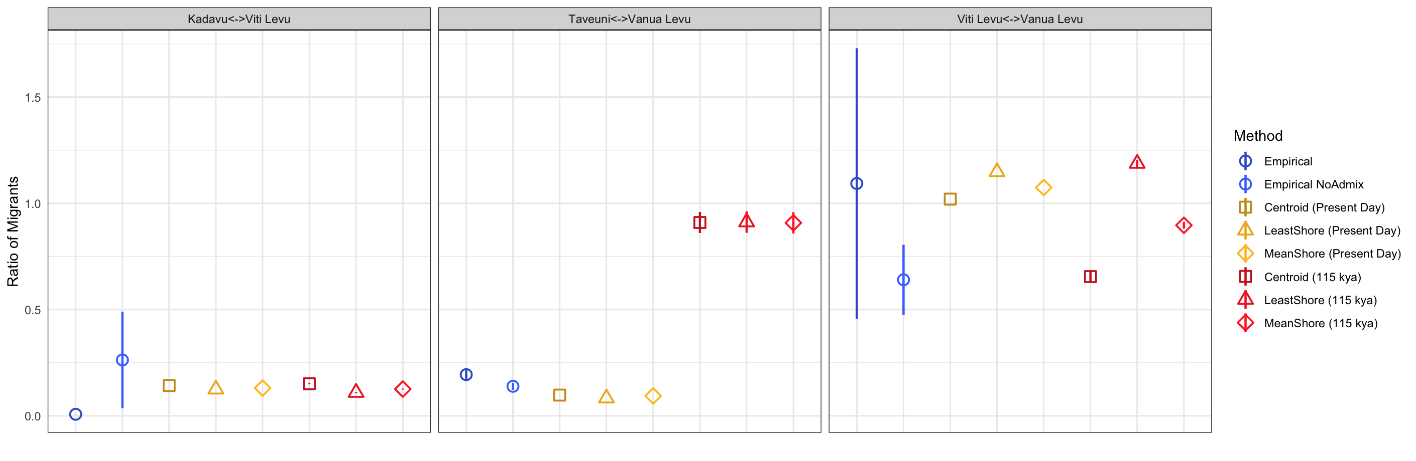
The results of the reanalysis show that empirical ratios of migrants for $\frac{Kadavu \to Viti Levu}{Viti Levu \to Kadavu}$ broadly correspond with neutral expectations from MacArthur & Wilson (1967), and suggest that the expected net migration rates are unlikely to have changed much over the last 115,000 years. In contrast, empirical migration ratios for $\frac{Taveuni \to Vanua Levu}{Vanua Levu \to Taveuni}$ seem to be much more consistent with neutral expectations based on present day sea levels rather than net migration expectations averaged over the last 115,000 years of sea level change. The empirical net migration ratios for $\frac{Viti Levu \to Vanua Levu}{Vanua Levu \to Viti Levu}$ are a bit more challenging to interpret given the broad confidence intervals. However, it is worth noting that the neutral migration ratio expectations based on present-day geography are close to the mean migration ratio value inferred from empirical UCE data based on an admixture models. In contrast, the mean empirical migration ratio based on non-admixture models is roughly the same as the value inferred from the centroid-to-centroid distance model averaged over 115,000 years of sea level change. The results of this analysis show how PleistoDist can be used to generate neutral expectations of net migration between island pairs, which can be compared with empirical estimates derived from genome-wide data.

References

Gyllenhaal EF, Mapel XM, Naikatini A, Moyle RG, Andersen MJ. 2020. A test of island biogeographic theory applied to estimates of gene flow in a Fijian bird is largely consistent with neutral expectations. Mol. Ecol. [Internet] 29:4059–4073. Available from: http://dx.doi.org/10.1111/mec.15625

Last updated on Aug 23, 2022